From Warehouse to Dashboard: the BI Semantic Layer (Power BI)

A perfect star schema that nobody can use is a failure, and we've seen a few. The last mile between warehouse tables and a manager's screen is the semantic layer, a model that knows how tables relate, what "Net Sales" means, how to format rupees, and which rows each user may see. In Power BI this is the dataset (now called a semantic model). In Looker it's LookML. In Tableau it's the published data source. We'll use Power BI, because that's what most Pakistani employers ask for, but the ideas carry straight across.

What the semantic layer adds

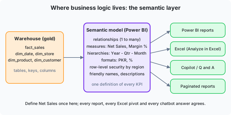
The warehouse gives you tables, keys and columns. The semantic layer adds:

• Relationships. Which key joins which, and in which direction filters flow (dimension to fact, one-to-many).
• Measures. Named calculations written once. Net Sales, Margin %, Sales YTD, Return Rate. A report author drags "Margin %" onto a chart and never sees the formula.
• Hierarchies. Year to Quarter to Month to Day, Category to Subcategory to SKU, so drill-down is one click.
• Formatting and names. "net_amount" becomes "Net Sales (PKR)" with thousands separators, and ugly key columns are hidden.
• Row-level security (RLS). The Lahore regional manager opens the same report as the CEO and sees only Lahore, enforced by a filter tied to their login.
• Descriptions and synonyms. So natural-language Q and A and Copilot know that "revenue" means Net Sales.

Because all of this lives in one model, every report, Excel pivot and chatbot answer built on it agrees. Business logic in the semantic layer is defined once. Business logic scattered across 40 report files is the "three numbers in one meeting" problem from Lesson 1 coming back through the side door.

The star schema inside Power BI

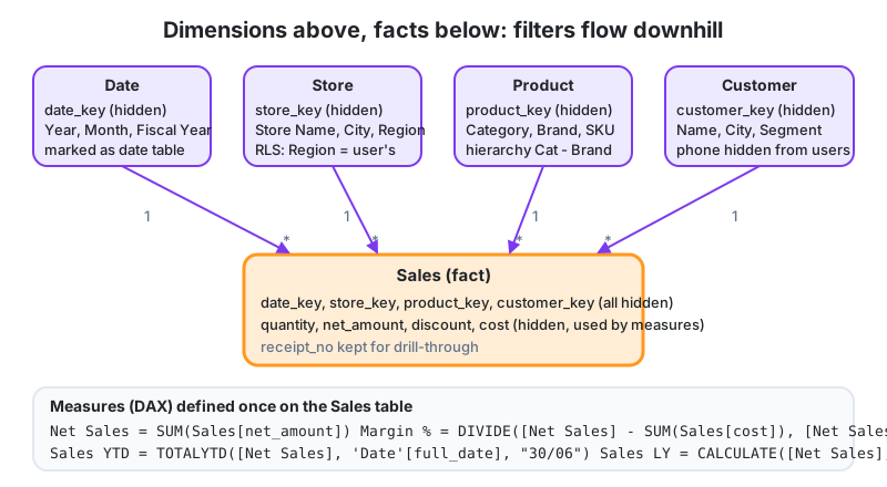
Power BI's engine (VertiPaq, columnar and in-memory) is built for stars. The recommended layout, shown in the diagram, is dimensions on top, fact below, all relationships one-to-many from dimension to fact with single-direction filtering. The practices below follow directly from this track, and they're the ones we check first when a student's model gives odd totals.

Practice	Why
Import gold star-schema tables, not source tables or wide flat extracts	Small, fast model; relationships are obvious; measures aggregate correctly
Hide all surrogate key columns	Users never group by an integer key
Mark dim_date as the date table	Enables time-intelligence functions
Avoid bidirectional relationships and many-to-many	Ambiguous filters and wrong totals; use bridge tables in the warehouse instead
No calculated columns for business logic; use measures	Calculated columns bloat the model; measures respond to filters
Prefer Import mode; use DirectQuery only for very large or real-time facts	Import is far faster; DirectQuery pushes every click to the warehouse

Measures on the retail star

-- DAX measures defined once on the Sales table

Net Sales = SUM ( Sales[net_amount] )

Cost of Sales = SUM ( Sales[cost] )

Gross Margin = [Net Sales] - [Cost of Sales]

Margin % = DIVIDE ( [Gross Margin], [Net Sales] )

Sales YTD (Fiscal) = TOTALYTD ( [Net Sales], 'Date'[full_date], "30/06" )

Sales LY = CALCULATE ( [Net Sales], SAMEPERIODLASTYEAR ( 'Date'[full_date] ) )

YoY % = DIVIDE ( [Net Sales] - [Sales LY], [Sales LY] )

Return Rate % = DIVIDE ( SUM ( Returns[refund_amount] ), [Net Sales] )

-- Row-level security role "Regional Manager" on the Store table:
[region] = LOOKUPVALUE ( UserRegion[region], UserRegion[email], USERPRINCIPALNAME () )

Three things to notice. DIVIDE handles division by zero. Return Rate % combines two fact tables and only works because both share the conformed Date, Store and Product dimensions (Lesson 9). The RLS rule uses a small mapping table of email to region loaded from HR, so security follows the organisation chart on its own. Keep that mapping table in the warehouse, not in a spreadsheet someone emails around, or a regional manager will still be seeing the old region six months after a transfer.

Where does each piece of logic belong?

Logic	Warehouse (SQL)	Semantic layer (DAX)
Cleansing, keys, SCD, grain	Yes	Never
Row-level additive facts (net = gross - discount)	Yes, as a column	No
Aggregations and ratios that depend on filters (margin %, YoY)	No	Yes, as measures
Daily aggregate tables for speed	Yes, in gold	Or Power BI aggregations
Security by region	Views or column masking for SQL users	RLS for report users

The rule of thumb is simple. Anything that's true about a row goes in the warehouse. Anything that depends on what the user has filtered goes in a measure.

Sixty reports, sixty margins: a Faisalabad textile group had 60 Power BI reports built by different analysts, each with its own "Gross Margin" formula (some included freight, some didn't). The CFO stopped trusting any of them. The BI team published one certified semantic model on the warehouse's gold star schema, with 40 measures and RLS by business unit, and rebuilt the top 12 reports on it as thin reports. Excel users connected to the same model. Within a quarter, "which margin is this?" stopped being asked in the monthly review. It's the order we teach on our Power BI course too, model first and reports second.

Quick recap

• The semantic layer turns warehouse tables into a governed model. Relationships, measures, hierarchies, formats, security and descriptions, defined once.
• Build it on the gold star schema with one-to-many single-direction relationships, keys hidden and the date table marked.
• Row-level truths go in SQL. Filter-dependent calculations go in DAX measures, not calculated columns.
• One certified model with thin reports on top ends the "which number is right?" problem for good.

Assignments

1. Write DAX measures for Units Sold, Average Selling Price (units and amount from Sales) and Average Basket Value (needs a distinct count of receipt_no).
2. Decide for each whether it's a warehouse column or a DAX measure: discount amount per line; discount percentage of sales; month-to-date units; product cost.
3. Design the RLS for a school network where principals see their campus, area heads see several campuses, and the CEO sees all. What mapping table do you need?