Warehouse Performance: Partitioning, Indexing, Columnar Storage

A compliance query that took 40 minutes. A dashboard that timed out every Monday morning. A BigQuery bill nobody could explain. Every one of those we've fixed came down to the same three ideas, and none of them needed new hardware. A warehouse query touches millions of rows by design, so the tricks that make an OLTP database fast (a B-tree index and a single-row seek) mostly don't apply. Warehouse speed comes from reading fewer bytes per row (columnar storage), reading fewer rows (partition pruning and clustering), and reading them fewer times (aggregates and caching).

Columnar storage

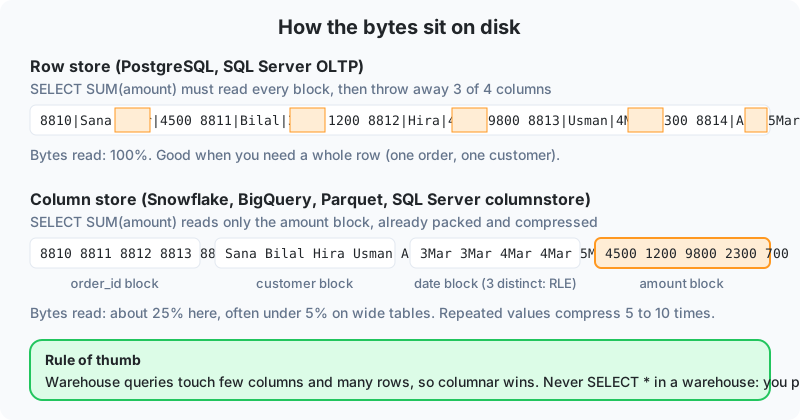
In a row store every row's values sit together. In a column store every column's values sit together. For SUM(net_amount) over 50 million rows and 25 columns, a row store reads all 25 columns (100 percent of the table) and a column store reads one (about 4 percent). On top of that, values in one column look alike, so they compress extremely well. A column of 50 million date keys with only 1,095 distinct values might shrink 20 times with run-length and dictionary encoding. Less I/O and less memory means faster queries, and on BigQuery it directly means a smaller bill.

All the cloud warehouses from Lesson 14 are columnar. SQL Server and PostgreSQL offer it as an option (clustered columnstore indexes, and extensions such as Citus columnar). Three practical rules follow.

• Never SELECT * from a fact table. Name the columns.
• Keep fact tables narrow. Text belongs in dimensions.
• Load in large batches. Columnar engines rebuild compressed segments, so thousands of single-row inserts are slow and leave fragmentation behind.

Partitioning

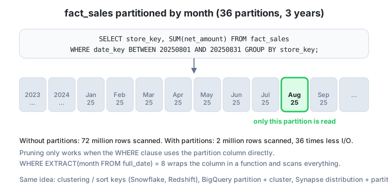
A partitioned table is physically split into pieces by the value of one column, almost always the date. A query with WHERE date_key BETWEEN 20250801 AND 20250831 reads only the August partition, 1/36th of a three-year table. This is partition pruning, and it's the single biggest speed-up available on large facts. It also makes maintenance easy. Reload one month, or drop the oldest year, by touching one partition.

Pruning only works when the filter is on the partition column itself, in a form the optimiser can compare. WHERE EXTRACT(MONTH FROM full_date) = 8 wraps the column in a function and scans everything. Filter on date_key or sale_date directly, and teach your BI tool to do the same (a date slicer on the marked date table does). Nine times out of ten, the slow query a client sends us has a function wrapped around the partition column.

Clustering and sort keys

Within a partition, data can be ordered so related rows sit together. Snowflake calls it clustering keys, Redshift sort keys, BigQuery clustering, SQL Server columnstore segment ordering. If the fact is clustered by store_key, a query for one store skips most blocks, because each block records its minimum and maximum store key (a "zone map") and blocks outside the range are never read. Pick one or two columns that appear in most filters, typically date and the most-filtered dimension key.

Distribution (MPP engines)

Massively parallel engines (Synapse dedicated pools, Redshift, Teradata) spread each table across many nodes. A join is fast when matching rows live on the same node. The common pattern is to distribute the big fact by a high-cardinality key (customer, or a hash of the receipt) and replicate small dimensions to every node so any join is local. Get this wrong and every query shuffles data across the network. Snowflake and BigQuery handle it automatically.

Indexes: a smaller role

Index type	OLTP use	Warehouse use
B-tree on primary key	Essential	Useful on dimension surrogate keys; rarely on facts (columnar engines ignore or replace it)
B-tree on a filter column	Common	Replaced by partitioning and clustering
Columnstore index	Rare	The main storage format on SQL Server warehouses
Bitmap index	Rare	Oracle warehouses, for low-cardinality flags

On PostgreSQL used as a small warehouse, do index the fact's foreign keys and date column, and partition by month, because PostgreSQL is a row store and those indexes are what it has.

Aggregates and caching

If 200 store managers open the same "yesterday by hour" page every morning, computing it from 2 million line items 200 times is waste. Build a gold aggregate table (store by hour by day) in the nightly load and point the dashboard at it. Most engines also cache query results, so an identical query on unchanged data returns instantly. Power BI import mode is itself a cache. It reads the warehouse once per refresh, not once per click.

A PostgreSQL fact table built for speed

-- Partition the fact by month on the integer date key
CREATE TABLE dw.fact_sales (
  date_key INT NOT NULL, store_key INT NOT NULL, product_key INT NOT NULL,
  customer_key INT NOT NULL, receipt_no TEXT NOT NULL, line_no SMALLINT NOT NULL,
  quantity INT NOT NULL, net_amount NUMERIC(12,2) NOT NULL, cost NUMERIC(12,2) NOT NULL
) PARTITION BY RANGE (date_key);

CREATE TABLE dw.fact_sales_2025_08 PARTITION OF dw.fact_sales
  FOR VALUES FROM (20250801) TO (20250901);
CREATE TABLE dw.fact_sales_2025_09 PARTITION OF dw.fact_sales
  FOR VALUES FROM (20250901) TO (20251001);

-- Indexes on the join keys (row store, so these matter here)
CREATE INDEX ON dw.fact_sales (store_key);
CREATE INDEX ON dw.fact_sales (product_key);

-- Check pruning: only fact_sales_2025_08 should appear in the plan
EXPLAIN
SELECT store_key, SUM(net_amount)
FROM dw.fact_sales
WHERE date_key BETWEEN 20250801 AND 20250831
GROUP BY store_key;

-- Daily aggregate for the dashboard, rebuilt nightly
CREATE MATERIALIZED VIEW mart_sales.daily_store_hour AS
SELECT f.date_key, f.store_key, t.hour_of_day,
       COUNT(DISTINCT f.receipt_no) AS receipts,
       SUM(f.quantity) AS units, SUM(f.net_amount) AS net_sales
FROM dw.fact_sales f
JOIN dw.dim_time t ON t.time_key = f.time_key
GROUP BY f.date_key, f.store_key, t.hour_of_day;

REFRESH MATERIALIZED VIEW mart_sales.daily_store_hour;

A performance checklist

1. Is the fact partitioned by date, and does the query filter on the partition column directly?
2. Is the table clustered or sorted by the most common filter key?
3. Does the query select only the columns it needs?
4. Are dimensions small enough to be broadcast or replicated, and are keys integers?
5. Is the dashboard reading an aggregate for repeated summary views?
6. Are loads batched, and are statistics refreshed after loading?
7. Does the query plan (EXPLAIN) confirm pruning and no unexpected full scans?

Forty minutes to twelve seconds, no new hardware: a wallet-scale fact table held 1.4 billion transactions. A compliance report, "transactions above PKR 500,000 for one CNIC in the last 90 days", took 40 minutes. The table was partitioned by month, but the query filtered on TO_DATE(date_key::TEXT, 'YYYYMMDD') >= CURRENT_DATE - 90, which defeated pruning. Rewriting the filter as date_key >= 20250516 (computed in the application) and adding a clustering key on account_key brought it to 12 seconds.

The whole lesson in one habit

Read the query plan. Most slow warehouse queries are one wrong filter away from fast. The rest is short. Fewer bytes (columnar, narrow selects), fewer rows (partition pruning, clustering), fewer reads (aggregates, caching). Filter on the partition column directly. On MPP engines distribute facts and replicate dimensions. B-tree indexes matter on row-store warehouses like PostgreSQL and far less on columnar engines.

Drill

1. Rewrite so that partition pruning works: WHERE TO_CHAR(full_date, 'YYYY-MM') = '2025-08' on a fact partitioned by date_key.
2. A fact has 40 columns, 200 million rows, and a dashboard query selects 4 columns. Estimate the fraction of bytes read on a row store versus a column store, ignoring compression.
3. Propose partition, cluster and aggregate choices for a K-Electric fact_meter_reading table (one row per meter per day, 3 million meters) that serves a "units by feeder by month" dashboard.