Data Lake, Lakehouse and the Medallion Architecture

Around 2010 the warehouse got a rival. Companies were collecting web logs, sensor readings, images and JSON from apps, none of which fitted neatly into fact and dimension tables, and storing all of it in a warehouse was expensive. The data lake was the answer. Dump everything as files on cheap storage and sort it out later. It solved one problem and created another, and the lakehouse with its medallion architecture is the current attempt to get the best of both. Three terms, one lesson, and job adverts should make more sense afterwards.

Lake, warehouse, lakehouse

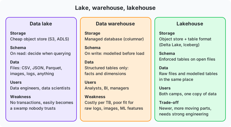
	Data lake	Data warehouse	Lakehouse
Storage	Object storage (S3, Azure Data Lake Storage, GCS)	Managed columnar database	Object storage plus an open table format
Schema	On read: files are whatever they are; structure is imposed at query time	On write: modelled before loading	Enforced schema on top of open files
Data types	Anything: CSV, JSON, Parquet, images, audio, logs	Structured tables only	Raw files and modelled tables side by side
Transactions	None; a half-written folder is a real risk	Full ACID	ACID via Delta Lake, Apache Iceberg or Apache Hudi
Main users	Data engineers, data scientists	Analysts, BI, managers	Both, on one copy of the data
Failure mode	The "data swamp": thousands of files nobody documents or trusts	Cost and rigidity; raw and unstructured data left out	Complexity; needs disciplined engineering
Typical tools	Hadoop, Spark, Athena, raw S3	Snowflake, BigQuery, Synapse, Redshift	Databricks, Microsoft Fabric, Snowflake with Iceberg, BigLake

The technical enabler of the lakehouse is the open table format. Delta Lake and Iceberg add a transaction log on top of Parquet files, which gives you ACID updates, schema enforcement, time travel (query the table as it was last Tuesday) and the ability to run MERGE statements on files sitting in cheap storage. That's what lets one copy of the data serve both a Spark machine-learning job and a Power BI dashboard.

The medallion architecture

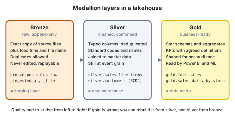
Databricks popularised a naming scheme for lakehouse layers, and it maps almost exactly onto the staging, core and mart layers from Lesson 3.

Bronze (raw)

Files and tables exactly as ingested, append-only, with ingestion metadata (load timestamp, source file, batch ID). Duplicates and bad rows are allowed. Bronze is never edited. It's the replayable history that makes ELT possible, the equivalent of a permanent staging archive.

Silver (cleaned and conformed)

Typed, deduplicated, validated, with standard codes and master-data keys applied, still at event grain. Silver is where the SCD Type 2 customer table and the line-item sales table live. The equivalent of the core warehouse.

Gold (business-ready)

Star schemas, aggregates and KPI tables with agreed definitions, shaped for a specific audience and read by BI tools and ML features. The equivalent of data marts. Some teams add a "platinum" or "semantic" layer for the Power BI model itself.

The rule that keeps a lakehouse from turning into a swamp is the same one that keeps a warehouse honest. Each layer is derived only from the layer before it, and consumers read only from gold (or, for data scientists, silver). The swamps we've been called in to drain all broke that rule within the first year.

Medallion in SQL (Spark or Fabric style)

-- Bronze: land the raw POS export as-is, append-only
CREATE TABLE bronze.pos_sales_raw (
  txn_no STRING, shop STRING, dt STRING, item STRING, qty STRING, amt STRING,
  _ingested_at TIMESTAMP, _source_file STRING
) USING DELTA;

COPY INTO bronze.pos_sales_raw
FROM 'abfss://landing@retaildl.dfs.core.windows.net/pos/2025-08-14/'
FILEFORMAT = CSV FORMAT_OPTIONS ('header' = 'true');

-- Silver: clean, type and deduplicate with a merge
MERGE INTO silver.sales_line_items t
USING (
  SELECT DISTINCT
         txn_no                                        AS receipt_no,
         TRIM(shop)                                    AS store_code,
         TO_TIMESTAMP(dt, 'dd/MM/yyyy HH:mm')          AS sold_at,
         item                                          AS sku,
         CAST(qty AS INT)                              AS quantity,
         CAST(REPLACE(amt, ',', '') AS DECIMAL(12,2))  AS net_amount
  FROM bronze.pos_sales_raw
  WHERE _ingested_at >= current_date()
) s
ON t.receipt_no = s.receipt_no AND t.sku = s.sku
WHEN MATCHED THEN UPDATE SET *
WHEN NOT MATCHED THEN INSERT *;

-- Gold: the star-schema fact, keys resolved
CREATE OR REPLACE TABLE gold.fact_sales AS
SELECT CAST(date_format(s.sold_at, 'yyyyMMdd') AS INT) AS date_key,
       st.store_key, p.product_key,
       s.receipt_no, s.quantity, s.net_amount
FROM silver.sales_line_items s
JOIN gold.dim_store   st ON st.store_code = s.store_code
JOIN gold.dim_product p  ON p.sku = s.sku AND p.is_current;

-- Time travel: what did silver look like before today's load?
SELECT COUNT(*) FROM silver.sales_line_items VERSION AS OF 41;

Nothing conceptually new happened. Staging, cleansing, SCD lookups, star schema. The difference is that all three layers are files in object storage with a transaction log, so the same tables are readable by Python notebooks, SQL endpoints and Power BI without copying. One practical note from Fabric projects. VERSION AS OF time travel is wonderful for debugging, and it's also why the storage bill keeps growing until someone schedules a VACUUM.

When to choose what

• Pure warehouse. Structured sources only, BI is the main consumer, the team is SQL-focused. Most small and mid-size Pakistani companies.
• Lake plus warehouse. Raw and unstructured data land in a lake; curated tables are loaded into a warehouse for BI. Common in banks and telcos today.
• Lakehouse. Significant ML or semi-structured data, a data engineering team comfortable with Spark or Fabric, and a wish to avoid keeping two copies. Growing fast with Microsoft Fabric adoption.

Six months of call records, exported every time: a Pakistani telecom operator kept call detail records (billions of rows) in a Hadoop lake and a customer warehouse on Teradata. Every churn model needed a copy of six months of CDRs exported into the warehouse, a two-day job. After moving to a lakehouse with Delta tables, the churn features (silver) and the BI star schema (gold) are computed from the same bronze CDR files, and the export step vanished. The finance team still sees a star schema in Power BI and never learned the word Parquet, which is how it should be.

The recap

• A lake stores any file cheaply with schema on read. A warehouse stores modelled tables with schema on write. A lakehouse enforces tables on open files with ACID.
• Open table formats (Delta, Iceberg) add transactions, schema enforcement and time travel to object storage.
• Bronze, silver, gold equals staging, core, marts, with the same layering rules. Consumers read gold.
• Choose by data types, consumers and team skills. The dimensional model is the same in all three.

Three tasks

1. Classify each into bronze, silver or gold: raw courier API JSON; deduplicated shipments with typed columns; daily on-time delivery percentage by city.
2. Explain "schema on read" versus "schema on write" using a CSV of school results that has an extra column in half the files.
3. A manager asks whether to move a 300 GB SQL Server warehouse to a lakehouse. List three questions you'd ask before answering.