Dimensionality Reduction: PCA

A student once brought us a customer table with 96 columns and asked why k-means was giving her nonsense. Units sold and revenue, calls and minutes, height and weight: half the columns were saying the same thing twice. Redundant columns slow models down, confuse anything distance-based and make plots impossible. Principal Component Analysis (PCA) finds a small set of new axes that hold most of the information, so 40 columns can become 5 with very little lost. It's the standard first step before clustering wide data and the standard way to draw a 2-D picture of it.

The idea in one picture

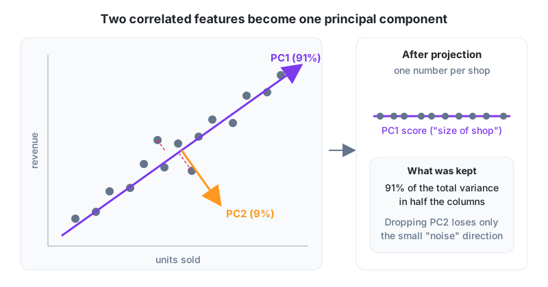
PCA rotates the axes. The first principal component (PC1) is the direction along which the data spreads the most. PC2 is the next-most-varying direction at right angles to PC1, and so on. Each component is a weighted mix of the original columns. Project every row onto the first few components and you get new, uncorrelated features ordered by how much variance they carry.

Two features into one, by hand

Five shops, features already standardised (mean 0, so we can skip the centring step).

Shop	x = units (z)	y = revenue (z)	p1 = (x + y) / sqrt(2)	p2 = (x - y) / sqrt(2)
1	-1.4	-1.2	-1.84	-0.14
2	-0.7	-0.9	-1.13	0.14
3	0.0	0.2	0.14	-0.14
4	0.7	0.6	0.92	0.07
5	1.4	1.3	1.91	0.07

Because x and y rise together, the natural axes are the diagonal (x + y) and the anti-diagonal (x - y); dividing by sqrt(2) keeps the axes unit length. Now compare variances (mean of squares, since means are 0):

• var(x) = (1.96 + 0.49 + 0 + 0.49 + 1.96) / 5 = 0.98
• var(y) = (1.44 + 0.81 + 0.04 + 0.36 + 1.69) / 5 = 0.87
• Total variance = 1.85
• var(p1) = (3.39 + 1.28 + 0.02 + 0.85 + 3.65) / 5 = 1.84
• var(p2) = (0.02 + 0.02 + 0.02 + 0.005 + 0.005) / 5 = 0.014

The total hasn't changed (1.84 + 0.014 = 1.85, because a rotation neither creates nor destroys variance), but now PC1 holds 1.84 / 1.85 = 99.2% of it. Keep only p1 and you've halved the columns while losing under 1% of the information. On real data the exact directions come from the eigenvectors of the covariance matrix. The library does that arithmetic; the logic is exactly what you just did.

How many components to keep

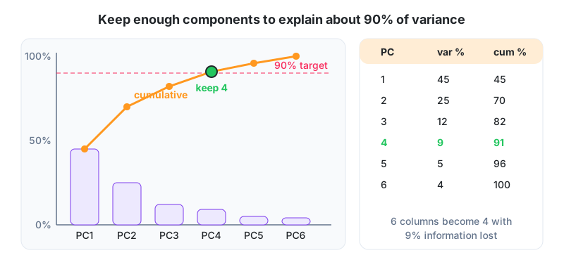
Plot the explained variance ratio per component (the scree plot) and its running total. The usual rules: keep enough for 90 to 95% cumulative variance, or stop at the elbow, or keep two if all you want is a picture. In the diagram, four of six components reach 91%.

Habits that keep PCA honest

Do	Because
Standardise first	otherwise the column with the biggest units becomes PC1 by default
Fit PCA on training data only	the rotation is a learned transformation; leaking test rows inflates scores
Read the loadings	the weights of each original column in a component tell you what it means ("size of shop", "payment risk")
Keep the original features for interpretation	a coefficient on PC3 means nothing to a manager
Use it for visualisation, noise reduction, and speeding up distance-based models	tree models rarely benefit; they handle redundant columns fine

PCA captures only linear structure. For curved manifolds and pretty 2-D maps of high-dimensional data, t-SNE and UMAP are the usual next tools, but they're for looking at, not for feeding into a model. We've had to talk more than one student out of training on t-SNE coordinates.

# run locally
import numpy as np
from sklearn.preprocessing import StandardScaler
from sklearn.decomposition import PCA

Xs = StandardScaler().fit_transform(X_train)
pca = PCA().fit(Xs)
ratio = pca.explained_variance_ratio_
print(np.round(ratio, 3))
print(np.round(np.cumsum(ratio), 3))           # find where it crosses 0.90

k = int(np.argmax(np.cumsum(ratio) >= 0.90)) + 1
pca_k = PCA(n_components=k).fit(Xs)
Z_train = pca_k.transform(Xs)                  # new features, k columns
loadings = pca_k.components_[0]               # weights of PC1 on original columns
for name, w in sorted(zip(X_train.columns, loadings), key=lambda t: -abs(t[1]))[:5]:
    print(name, round(w, 2))

96 columns down to 6 at a power utility: A load-analytics team had 96 columns per customer, energy use in each 15-minute slot of a typical day. Clustering on all 96 gave noisy groups nobody could explain. PCA cut them to 6 components holding 93% of the variance. PC1 loaded on total daily use ("size"), PC2 set evening use against daytime use ("residential vs commercial pattern"), PC3 caught a midday air-conditioning peak. k-means on those 6 components produced clean tariff segments, and a single scatter of PC1 against PC2 let the team show management residential, commercial and industrial customers visibly pulling apart.

Quick recap

• PCA rotates to new uncorrelated axes ordered by variance, and the first few usually hold most of the information.
• Total variance is preserved. The scree plot tells you how much to keep (90 to 95% is typical).
• Standardise first and fit on training data only.
• Loadings tell you what each component means. Use them, and keep the raw features for reporting.
• It helps distance-based models and plots. It rarely helps tree models.

Try this before the next lesson

1. Project a new shop with (x, y) = (0.5, -0.5) onto p1 and p2. Which component carries its information, and what does that say about the shop?
2. A scree plot shows ratios 0.52, 0.21, 0.11, 0.07, 0.05, 0.04. How many components are needed for 90%? For 95%?
3. Explain in two sentences why you shouldn't run PCA before a random forest just to "speed it up" if you also need feature importances.