"Fit a line to these five points and tell me the slope." We've had students report exactly that question from a Lahore fintech interview, pen and paper, no laptop. Linear regression is the algorithm you learn first not because it's the most accurate but because everything after it is a variation on the same three ideas: a formula with parameters, a loss that measures error, and a procedure that adjusts the parameters to shrink the loss. Fit a line by hand once and gradient boosting stops looking like magic.

The model

With one feature the model is a straight line, y = b0 + b1 x. b0 is the intercept (the prediction when x = 0) and b1 is the slope (how much y moves when x rises by one unit). With several features it becomes y = b0 + b1 x1 + b2 x2 + ... and each b is the effect of its feature with the others held fixed.

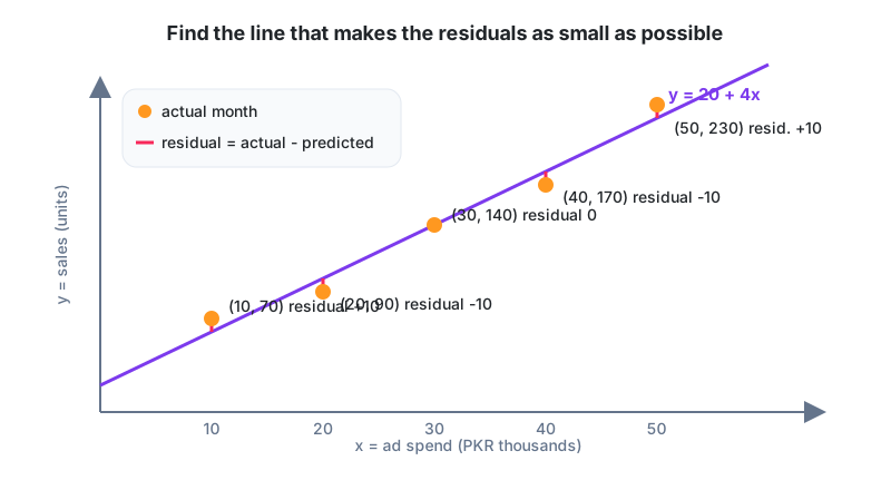
A residual is actual minus predicted for one row. The best line minimises the sum of squared residuals. Squared, so positive and negative misses don't cancel and big misses hurt more.

Fit the line with a pen

Five months of a Lahore clothing brand's Facebook ad spend (x, PKR thousands) and units sold (y).

Month	x	y	x - 30	y - 140	(x - 30)(y - 140)	(x - 30)^2
1	10	70	-20	-70	1,400	400
2	20	90	-10	-50	500	100
3	30	140	0	0	0	0
4	40	170	10	30	300	100
5	50	230	20	90	1,800	400
Sum	150	700			4,000	1,000

The means are x-bar = 150 / 5 = 30 and y-bar = 700 / 5 = 140. The least-squares formulas are:

b1 = sum[(x - x-bar)(y - y-bar)] / sum[(x - x-bar)^2] = 4,000 / 1,000 = 4.0
b0 = y-bar - b1 x-bar = 140 - 4 x 30 = 20

So the model reads units = 20 + 4 x spend. Every extra PKR 1,000 of ads brings about 4 more units, and with zero ads the brand still sells about 20. Now check the fit.

x	y	Predicted 20 + 4x	Residual	Residual^2
10	70	60	+10	100
20	90	100	-10	100
30	140	140	0	0
40	170	180	-10	100
50	230	220	+10	100
			0	400

MSE = 400 / 5 = 80, so RMSE = 8.9 units. Total variation SST = sum of (y - 140)^2 = 4,900 + 2,500 + 0 + 900 + 8,100 = 16,400. R^2 = 1 - 400 / 16,400 = 0.976, meaning the line explains 97.6% of the variation in sales. A PKR 35,000 budget gets 20 + 4 x 35 = 160 units.

How the computer finds b0 and b1

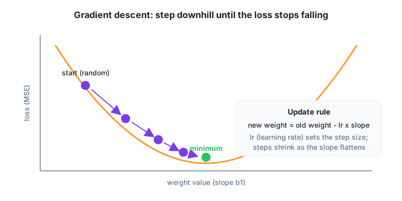
For a small problem the closed-form formula above is all you need. With many features and millions of rows, libraries use gradient descent: start with random parameters, compute the slope of the loss with respect to each one, step downhill, repeat.

Before you quote a coefficient

Check	Why
Scale features first if you want to compare coefficient sizes	a coefficient of 0.002 on "rupees" may matter more than 5 on "years"
Look at the residual plot	a curve in the residuals means the relationship is not linear; try log(x) or a polynomial term
Watch for multicollinearity	two near-identical features (units and revenue) make coefficients unstable
Correlation is not causation	ad spend rising before Eid does not prove ads caused Eid sales
Use ridge or lasso with many features	they shrink coefficients and prevent overfitting

# run locally
import numpy as np
from sklearn.linear_model import LinearRegression
from sklearn.metrics import mean_squared_error, r2_score

X = np.array([[10], [20], [30], [40], [50]])
y = np.array([70, 90, 140, 170, 230])
m = LinearRegression().fit(X, y)
print(m.intercept_, m.coef_)                  # 20.0 [4.0]
pred = m.predict(X)
print(np.sqrt(mean_squared_error(y, pred)))    # 8.94
print(r2_score(y, pred))                       # 0.976
print(m.predict([[35]]))                       # [160.]

Why the property agent chose the simpler model: An agent working Islamabad's Bahria Town wanted quick valuations. The analyst fitted a multiple regression on 900 recent sales with covered area (sq ft), plot size (marla), age of house, distance to the main gate and a one-hot phase indicator. It reached R^2 = 0.84 with an RMSE of about PKR 2.1 million on prices averaging 28 million. The coefficients turned out to be worth more than the score. Every extra marla added about PKR 1.9 million and every extra kilometre from the gate removed about 700,000, numbers the agent could quote to sellers. A gradient-boosting model later cut RMSE by 12% and was still turned down, because it couldn't produce those sentences.

Quick recap

Linear regression predicts a number with y = b0 + b1 x1 + ..., and the coefficients are readable effects.
The best line minimises the sum of squared residuals; with one feature you can compute it by hand.
RMSE is the typical error in the target's units. R^2 is the share of variation explained.
Gradient descent finds parameters when the formula is impractical.
Check residual plots, collinearity and causation before you quote a coefficient to anyone.

Interviewers love this lesson. "What does R^2 mean?", "why square the residuals?" and "what breaks when two features are nearly identical?" come up again and again, and we drill all three in our interview preparation sessions.

Try this before the next lesson

Add a sixth month (x = 60, y = 250) to the table and recompute b1 and b0 by hand. Does the slope move much?
Using units = 20 + 4 x spend, predict sales at spend 0 and at spend 200. Which prediction should you distrust, and why?
For a K-Electric model predicting monthly units from house size, number of ACs and month, write down what the coefficient on "number of ACs" means in plain words.

Linear Regression