Gradient Boosting (XGBoost, LightGBM)

Here's an opinion we'll defend in any classroom: on tabular business data, gradient boosting is the model to beat. It wins the competitions, and it's what banks and e-commerce companies actually ship as XGBoost, LightGBM or CatBoost. The idea is almost the opposite of a random forest. Instead of many independent trees voting, boosting grows small trees one after another, and each new tree is trained on the mistakes of everything before it.

The core idea

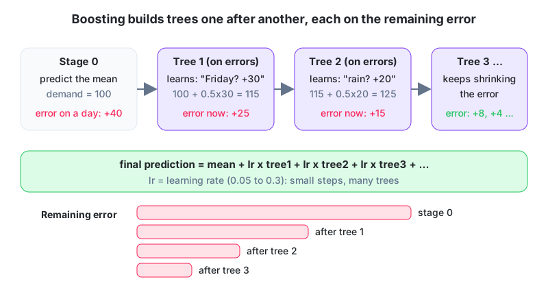
1. Start with a constant prediction, usually the mean of the target.
2. Compute the residual (actual minus current prediction) for every row.
3. Fit a small tree (depth 3 to 6) to predict those residuals.
4. Add the tree's output, shrunk by a learning rate, to the current prediction.
5. Repeat steps 2 to 4 for hundreds of trees, stopping when validation error stops improving.

The "gradient" in the name is there because residuals are the gradient of squared error. For classification the same machinery runs on the gradient of log loss, so the trees fit "how wrong was the probability" instead of "how wrong was the number".

Two rounds of boosting, by hand

Daily bread demand for a Rawalpindi bakery, four days, learning rate 0.5.

Day	Friday?	Rain?	Actual	F0 = mean	Residual r1
Mon	no	no	90	110	-20
Tue	no	yes	110	110	0
Fri	yes	no	130	110	+20
Fri (rain)	yes	yes	110	110	0

Mean = (90 + 110 + 130 + 110) / 4 = 110. Tree 1 is a single split on "Friday?": Friday rows have mean residual (+20 + 0) / 2 = +10; non-Friday rows have (-20 + 0) / 2 = -10. Update: F1 = F0 + 0.5 x tree1.

Day	Tree 1 output	F1	Residual r2
Mon	-10	110 - 5 = 105	-15
Tue	-10	105	+5
Fri	+10	115	+15
Fri (rain)	+10	115	-5

Tree 2 is fitted to the new residuals r2. A split on "Rain?" alone does not help (rainy rows average (+5 - 5) / 2 = 0 and dry rows average (-15 + 15) / 2 = 0), because rain and Friday interact. A depth-2 tree finds this: it splits on Rain first and then on Friday inside each branch, giving four leaves: dry non-Friday -15, rainy non-Friday +5, dry Friday +15, rainy Friday -5. Update F2 = F1 + 0.5 x tree2.

Day	Tree 2 output	F2	Actual	Error
Mon	-15	105 - 7.5 = 97.5	90	-7.5
Tue	+5	105 + 2.5 = 107.5	110	+2.5
Fri	+15	115 + 7.5 = 122.5	130	+7.5
Fri (rain)	-5	115 - 2.5 = 112.5	110	-2.5

Sum of squared error went from 800 (stage 0) to 500 (after tree 1) to 125 (after tree 2). Each round removes a large share of what's left, and the learning rate of 0.5 is why no single tree gets trusted fully. Tree 3 would fit these smaller residuals and shrink them again. Real models use a learning rate of 0.05 to 0.1 with several hundred trees, so the error falls in many small steps rather than a few big ones.

Bagging versus boosting

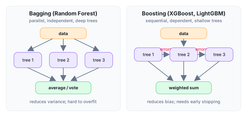
	Random forest (bagging)	Gradient boosting
Trees	deep, independent, parallel	shallow, sequential, each depends on the last
Reduces	variance	bias (and variance with shrinkage)
Overfitting risk	low; more trees never hurt	real; too many trees overfit, use early stopping
Tuning effort	little	moderate: learning rate, trees, depth, subsample, regularisation
Typical accuracy on tabular data	very good	usually the best

The knobs that matter

Parameter	Role	Starting point
learning_rate	shrinks each tree's contribution	0.05
n_estimators	number of trees; pair with early stopping	500 to 2000 with early stopping
max_depth / num_leaves	tree complexity	depth 4 to 6, or 31 leaves in LightGBM
subsample, colsample_bytree	random rows/columns per tree, limits overfitting	0.8
reg_lambda, min_child_weight	regularisation	1.0, 5
scale_pos_weight	up-weights the rare class	negatives / positives

# run locally: pip install lightgbm
import lightgbm as lgb
from sklearn.model_selection import train_test_split

X_tr, X_va, y_tr, y_va = train_test_split(X, y, test_size=0.2, stratify=y, random_state=0)
model = lgb.LGBMClassifier(learning_rate=0.05, n_estimators=2000, num_leaves=31,
                           subsample=0.8, colsample_bytree=0.8, random_state=0)
model.fit(X_tr, y_tr, eval_set=[(X_va, y_va)], eval_metric="auc",
          callbacks=[lgb.early_stopping(50)])
print("best iteration:", model.best_iteration_)
print("validation AUC:", model.best_score_["valid_0"]["auc"])

What 60 features and early stopping bought a wallet: A mobile wallet in Lahore replaced a logistic fraud model with LightGBM on 60 features (velocity counts, device changes, receiver history, time of day). On the same daily alert budget of 2,000 cases the boosted model caught 31% more confirmed fraud, mostly because it picked up interactions such as "new device AND first transfer to this receiver AND amount above the user's 30-day maximum" that a linear model can't express without hand-built interaction features. Early stopping settled at 640 trees, and training took four minutes on a laptop. What broke later was not the model but the feature service, which is a lesson 17 story.

If you remember one thing

Boosting adds shallow trees one at a time, each fitting the residuals of the model so far. A small learning rate, many trees and early stopping is the standard recipe, and it reduces bias while picking up interactions on its own, which is why it dominates tabular problems. Unlike a forest, more trees can overfit, so always validate. XGBoost, LightGBM and CatBoost are fast implementations of the same idea with different defaults; we teach LightGBM first because it's the quickest to train on a student laptop.

Homework

1. Redo the first boosting round with a learning rate of 1.0 instead of 0.5. What are F1 and the residuals r2? What is the danger?
2. Your boosted model has training AUC 0.99 and validation AUC 0.81 at 1,500 trees, and early stopping would have chosen 300. Name three settings you'd change.
3. For a K-Electric outage-prediction model, list two feature interactions you'd expect boosting to find on its own.