Case Studies and Practice: Churn, Fraud, Demand Forecasting

Here's a promise. If you can run the three projects in this lesson end to end, you can do the first year of most analyst jobs in Pakistan. Customer churn, transaction fraud and demand forecasting are the projects our graduates meet first, and for each we'll walk the CRISP-DM loop, choose the metric, sketch the features and work out the business value by hand. Treat them as templates for your own portfolio.

Case 1: telecom churn (classification, batch)

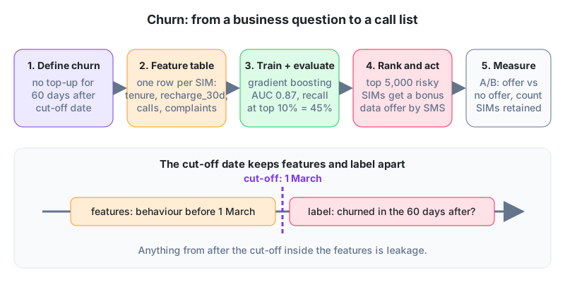
Step	Decision made
Business goal	each week, give the retention team the 5,000 prepaid SIMs most likely to go silent, to receive a bonus-data offer
Label	churned = no recharge in the 60 days after the cut-off date
Features (before cut-off)	tenure, recharges_30d, recharge_amount_90d, days_since_last_recharge, data_mb_30d trend, calls_to_helpline, complaints_90d, handset_age, city
Split	train on cut-offs Jan to Apr, validate on May, test on June (time-ordered)
Model	logistic baseline, then LightGBM with early stopping
Metric	precision in the top 5,000 (the list size), AUC for model comparison

Now the value calculation. Base churn rate is 8%. In the test month the model's top 5,000 contained 1,900 real churners (precision 38%, a lift of 4.75x over random). The offer costs PKR 150 per SIM and persuades 30% of contacted churners to stay, and a retained SIM is worth PKR 2,400 a year.

Item	Calculation	Value (PKR)
Offer cost	5,000 x 150	-750,000
Churners retained	1,900 x 30%	570 SIMs
Revenue saved	570 x 2,400	+1,368,000
Net per week		+618,000
Same with random list	400 churners x 30% x 2,400 - 750,000	-462,000

The model turns a loss-making campaign into a profitable one. That table goes on the first slide. The AUC goes in the appendix, if it goes anywhere.

Case 2: mobile-wallet fraud (classification, real time, imbalanced)

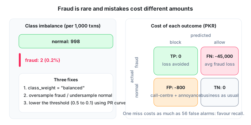
Step	Decision made
Business goal	block or step-up-verify transfers with high fraud risk in under 300 ms; investigators can review 2,000 alerts a day
Label	confirmed fraud from chargebacks and investigations (arrives up to 45 days late; training window ends 45 days ago)
Features	amount vs user's 30-day max, transfers_1h, distinct_receivers_24h, new_device, receiver_age_days, receiver_fraud_rate_to_date, hour, sim_swap_recent
Imbalance	0.2% positives: scale_pos_weight, stratified splits, PR-AUC as the tuning metric
Model	LightGBM, features computed by a streaming service; logistic model kept as fallback
Threshold	chosen from the cost matrix, not 0.5

Choosing the threshold from costs. Per 100,000 transactions there are 200 frauds. The average fraud loss is PKR 45,000, and a false alarm costs PKR 800 (a verification call plus an annoyed customer).

Threshold	Recall	Frauds caught	Frauds missed	False alarms	Loss from misses	Cost of alarms	Total cost
0.50	55%	110	90	300	4,050,000	240,000	4,290,000
0.20	78%	156	44	1,400	1,980,000	1,120,000	3,100,000
0.05	92%	184	16	6,000	720,000	4,800,000	5,520,000

Threshold 0.20 minimises total cost, and its 1,400 alarms per 100,000 transactions fit inside the investigators' capacity. Go lower and you catch more fraud while drowning both the team and the customers in false alarms. Notice that 0.5 never came into it.

Case 3: retail demand forecasting (regression, time series)

Step	Decision made
Business goal	weekly order quantity per product for a Lahore pharmacy chain of 40 branches; reduce stock-outs without raising expiry waste
Target	units sold per product per branch per week
Features	lags 1, 2, 4, 52; rolling mean and std 4 and 12; week of year; Eid and Muharram flags; dengue-season flag; price; promotion; branch type
Split	TimeSeriesSplit, last 12 weeks as test
Baselines	seasonal naive and 4-week moving average
Model	one LightGBM across all product-branch pairs with product and branch as categorical features
Metric	MAE in units (what the buyer feels) and MAPE for comparison across products

From forecast to order quantity. For one product the forecast for next week is 120 units with a residual std of 15 over the last 12 weeks. To keep the stock-out probability near 5%, order forecast + 1.65 x std = 120 + 24.75 = 145 units. A better forecast lowers the std and therefore the safety stock. Cutting std from 15 to 10 saves about 8 units of buffer per week for this product, multiplied across 3,000 product-branch pairs.

What all three have in common

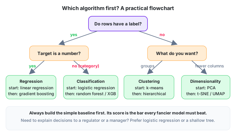
Lesson	Churn	Fraud	Demand
Define the label with a cut-off	60 days after cut-off	confirmed, 45-day lag	next week's units
Split matches reality	by time	by time, stratified	by time
Beat a baseline	"longest since recharge" rule	existing rules engine	seasonal naive
Metric = business capacity	precision at 5,000	cost at 2,000 alerts/day	MAE and safety stock
Deploy to fit the decision	weekly batch	real-time API	weekly batch

# run locally: a reusable project skeleton
from sklearn.pipeline import Pipeline
from sklearn.compose import ColumnTransformer
from sklearn.preprocessing import OneHotEncoder, StandardScaler
from sklearn.linear_model import LogisticRegression
from sklearn.metrics import roc_auc_score, precision_score
import numpy as np

def top_k_precision(y_true, scores, k):
    idx = np.argsort(scores)[::-1][:k]
    return float(np.asarray(y_true)[idx].mean())

prep = ColumnTransformer([("num", StandardScaler(), num_cols),
                          ("cat", OneHotEncoder(handle_unknown="ignore"), cat_cols)])
baseline = Pipeline([("prep", prep), ("clf", LogisticRegression(max_iter=2000))])
baseline.fit(X_train, y_train)
s = baseline.predict_proba(X_valid)[:, 1]
print("AUC", round(roc_auc_score(y_valid, s), 3),
      "precision@5000", round(top_k_precision(y_valid, s, 5000), 3))
# next: swap the "clf" step for LightGBM and compare on the same validation month

A first quarter on the job: One of our graduates joined a Lahore e-commerce company as its first data analyst. In her first quarter she shipped a weekly churn list (batch, logistic regression, precision at 3,000 of 29% against 9% for the old rule), then a return-risk score used to decide which cash-on-delivery orders needed a confirmation call, which saved about 400 failed deliveries a month. Neither used anything beyond this track. The fraud model came in year two, once enough confirmed cases existed. Her manager's summary was "she measured before she modelled, and she picked the metric we could act on".

Before you move on

• Every project starts with a decision, a capacity constraint and a label defined by a cut-off.
• Churn is batch classification measured by precision at the list size.
• Fraud is real-time, imbalanced classification with a threshold chosen from costs.
• Demand is time-series regression judged against seasonal naive and fed into a safety-stock rule.
• Translate every metric into rupees, hours or units before you present it.

When you've built one of these end to end and can defend every number in it, you're ready for the exam. Details are on our certification page.

Your portfolio homework

1. Recompute the churn value table if the offer cost rises to PKR 250 and the model's top-5,000 precision falls to 30%. Is the campaign still profitable?
2. In the fraud table, suppose the false-alarm cost drops to PKR 300 because verification becomes an automatic OTP. Which threshold now minimises total cost?
3. Pick a business you know (a school, a clinic, a shop, a ride service). Write a one-page project brief following the churn table: goal, label with cut-off, six features, split, baseline, metric and deployment mode.