k-Nearest Neighbours and Support Vector Machines

What do "customers like you bought this" and a spam filter have in common? Both are about distance between rows. k-nearest neighbours (kNN) has no training step at all; it memorises the data and, when asked, looks at the closest examples. A support vector machine (SVM) does the reverse and boils the whole dataset down to a handful of boundary points. Both are geometric, so both need scaled features, and the intuition you build here is the same one you'll need for clustering and PCA.

k-nearest neighbours

To classify a new row, kNN measures its distance to every training row, takes the k closest, and returns the majority label (or their average, for regression). That's the entire algorithm.

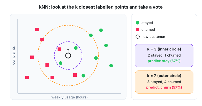
The diagram shows the catch. With k = 3 the vote says "stay"; with k = 7 it says "churn". Small k is flexible and noisy (it overfits), large k is smooth and may blur real boundaries (it underfits). Pick k with validation, and use an odd k for two classes so votes can't tie.

Classify one customer with k = 3

Features are already standardised (z-scores), weekly usage hours and complaints. The new customer is Q = (0.0, 0.5).

Customer	usage (z)	complaints (z)	Label	Euclidean distance to Q
1	0.4	0.3	stay	sqrt(0.16 + 0.04) = 0.45
2	-0.5	0.9	churn	sqrt(0.25 + 0.16) = 0.64
3	1.5	-1.0	stay	sqrt(2.25 + 2.25) = 2.12
4	-0.2	0.2	stay	sqrt(0.04 + 0.09) = 0.36
5	-1.2	1.4	churn	sqrt(1.44 + 0.81) = 1.50
6	0.9	1.1	churn	sqrt(0.81 + 0.36) = 1.08

Sorted distances: 0.36 (4, stay), 0.45 (1, stay), 0.64 (2, churn), 1.08, 1.50, 2.12. The three nearest are stay, stay, churn, so predict stay with probability 2/3. With k = 5 the vote is stay 2, churn 3, and the answer flips to churn. And this is why scaling matters. Had usage been in raw hours (0 to 60) and complaints in counts (0 to 5), the usage column alone would have decided every distance.

kNN strengths and costs

Good	Bad
No assumptions about the boundary shape	Prediction is slow: distance to every stored row
Trivial to understand and explain ("customers like you did X")	Weak with many features (distances become meaningless, the "curse of dimensionality")
Naturally multi-class	Sensitive to irrelevant features and to scaling

Support vector machines

An SVM looks for the boundary (a line in 2-D, a hyperplane in more dimensions) that separates the classes with the widest possible margin, the biggest empty street between the two groups. Only the points touching the edge of the street, the support vectors, decide where the boundary goes. Delete every other row and the model wouldn't change.

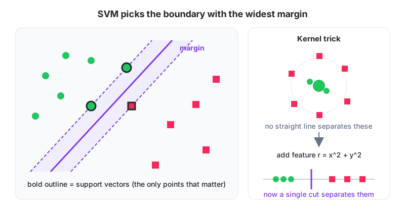
For a boundary w . x + b = 0, the margin width is 2 / ||w||, so maximising the margin means minimising ||w||. Real data overlaps, so a penalty C controls how much the model tolerates points inside the street or on the wrong side: large C = narrow margin, few mistakes on training data (risk of overfitting); small C = wide margin, more tolerance.

A quick numeric check. With w = (1, 1) and b = -3, the boundary is x1 + x2 = 3, ||w|| = sqrt(2) = 1.414, and the margin width is 2 / 1.414 = 1.41. A point (2.5, 1) gives 2.5 + 1 - 3 = +0.5, so it's on the positive side but inside the margin, a margin violation.

The kernel trick

Some classes can't be separated by a straight line, an inner ring and an outer ring for instance. Kernels let the SVM add features implicitly (x^2, x y, or infinitely many with the RBF kernel) so that a straight cut in the bigger space becomes a curved boundary in the original one. The right panel of the diagram shows the idea with r = x^2 + y^2. You choose the kernel (linear, polynomial, rbf) and its width gamma with validation, and in our experience rbf with default gamma is the right first try nine times out of ten.

# run locally
from sklearn.pipeline import make_pipeline
from sklearn.preprocessing import StandardScaler
from sklearn.neighbors import KNeighborsClassifier
from sklearn.svm import SVC
from sklearn.model_selection import cross_val_score

knn = make_pipeline(StandardScaler(), KNeighborsClassifier(n_neighbors=7))
svm = make_pipeline(StandardScaler(), SVC(kernel="rbf", C=1.0, gamma="scale"))
for name, m in [("kNN", knn), ("SVM", svm)]:
    scores = cross_val_score(m, X, y, cv=5, scoring="f1")
    print(name, scores.mean().round(3), scores.std().round(3))

When to use which

	kNN	SVM
Dataset size	small to medium (prediction cost grows with rows)	small to medium (training cost grows fast past ~100k rows)
Feature count	low (under 20)	works well even with many features, e.g. text
Explainability	show the neighbours	hard beyond linear kernel
Typical use	recommendation-style "similar customers", quick baselines	text classification, image features, small precise problems

Two projects, two different winners: A Daraz seller in Karachi wanted a suggested price for each new listing. We used kNN regression. Standardise brand, category, condition and specification features, find the 10 most similar existing listings, and average their selling prices. Sellers liked it because the app could show the ten comparable items ("phones like yours sold for PKR 38,000 to 42,000"). For a separate job classifying 20,000 customer-support messages into complaint types, an SVM with a linear kernel on TF-IDF text features reached 88% accuracy and trained in under a minute. kNN struggled there, because with thousands of word features every message looks equally far from every other.

Quick recap

• kNN predicts from the k closest training rows, and k sets the bias-variance trade-off.
• SVM finds the maximum-margin boundary defined only by the support vectors; C sets the tolerance.
• Kernels give SVMs curved boundaries without building the new features by hand.
• Both are distance-based, so scale the features first, every time.
• kNN is easy to explain and slow to predict. SVM is strong on high-dimensional data like text.

Try this

1. Using the six-customer table, classify a new point Q2 = (-0.6, 1.0) with k = 3. Show the three distances.
2. For w = (3, 4) and b = -10, compute ||w|| and the margin width. Which side is the point (1, 1) on?
3. Explain in two sentences why kNN with 200 features on 5,000 rows is likely to do badly, and what you could do about it.