Logistic Regression and Classification

Will this customer churn? Is this transfer fraud? Will this invoice be paid late? Most of what a business wants predicted is a yes or a no, and a straight line can't give you that. A line outputs any number at all, while a yes/no answer needs a probability between 0 and 1. Logistic regression fixes it with one trick, the sigmoid, and it's still the most widely deployed classifier in Pakistani banks and telcos because it's fast, stable and you can explain every score.

From a line to a probability

Logistic regression still computes a linear score, z = b0 + b1 x1 + b2 x2 + .... It then squashes z through the sigmoid, p = 1 / (1 + e^-z), which maps any z to a value between 0 and 1. Read that value as the probability of the positive class.

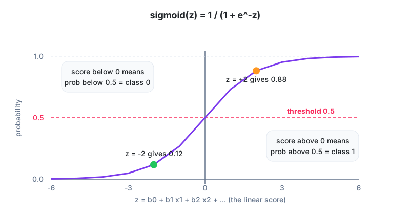
z	e^-z	p = 1 / (1 + e^-z)	Reading
-4	54.6	0.018	almost certainly class 0
-2	7.39	0.119	unlikely
0	1.00	0.500	coin flip
2	0.135	0.881	likely
4	0.018	0.982	almost certainly class 1

Score four customers with a calculator

A telecom in Peshawar fitted a churn model on two features, months since last recharge (m) and complaints in the last 90 days (c). The fitted equation is z = -2.0 + 0.6 m + 0.9 c.

Customer	m	c	z	e^-z	p(churn)	Predict at 0.5
A	1	0	-2.0 + 0.6 + 0 = -1.4	4.055	0.198	stay
B	4	1	-2.0 + 2.4 + 0.9 = 1.3	0.273	0.786	churn
C	2	2	-2.0 + 1.2 + 1.8 = 1.0	0.368	0.731	churn
D	0	0	-2.0	7.389	0.119	stay

What do the coefficients mean? Each one is a change in log-odds. e^0.6 = 1.82, so every extra month without a recharge multiplies the odds of churn by 1.82. e^0.9 = 2.46, so each complaint multiplies the odds by 2.46. Those are the sentences you hand the retention manager, and they're also what an interviewer means when they ask you to "interpret the model".

How the coefficients are learned

Instead of squared error, logistic regression minimises log loss. For a row with true label 1 the loss is -log(p); for label 0 it is -log(1 - p). Confident wrong answers get punished hard. For customer B above, if B really churned the loss is -log(0.786) = 0.24; if B stayed it is -log(0.214) = 1.54. Gradient descent adjusts the b values to reduce the total loss over all rows, just as in linear regression.

The threshold is a business decision

The model gives you a probability. Turning it into an action needs a cut-off, and 0.5 is only the default.

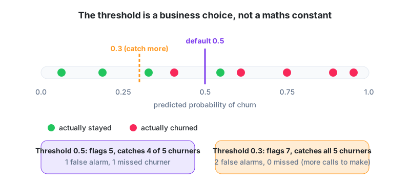
Lower the threshold when missing a positive is expensive (fraud, disease, churn of a high-value customer). Raise it when acting on a false alarm is expensive (blocking a legitimate payment, calling a happy customer). Lesson 14 shows how precision and recall move as you slide it.

Beyond two classes

For three or more classes (loan grade A/B/C), scikit-learn fits a softmax (multinomial) version that outputs one probability per class summing to 1. The interface is identical.

# run locally
import numpy as np
from sklearn.linear_model import LogisticRegression

X = np.array([[1, 0], [4, 1], [2, 2], [0, 0], [6, 0], [3, 3], [1, 1], [5, 2]])
y = np.array([0, 1, 1, 0, 1, 1, 0, 1])
clf = LogisticRegression().fit(X, y)
print(clf.intercept_, clf.coef_)              # b0, [b_m, b_c]
print(clf.predict_proba([[4, 1]])[:, 1])      # probability of churn
print(np.exp(clf.coef_))                      # odds multipliers per unit
threshold = 0.3
print((clf.predict_proba(X)[:, 1] >= threshold).astype(int))

When we reach for it, and when we don't

Choose it when	Look elsewhere when
You must explain each decision (State Bank audits, loan rejections)	Relationships are strongly non-linear and you cannot engineer the features
You have few rows relative to features	You have millions of rows and accuracy is everything (try gradient boosting)
You need calibrated probabilities for ranking	Features interact in complex ways (trees handle this natively)

A scorecard loan officers could defend: A microfinance lender in Multan needed credit scoring that its officers could explain to a customer's face. Logistic regression on eight features (income, existing loans, repayment history, business age, guarantor, district, and nothing gender-related) gave an AUC of 0.79. The odds ratios became a printed scorecard, with lines like "each previous late payment multiplies the risk of default by 2.1". Officers auto-approved below 0.35 and sent everything between 0.35 and 0.6 to manual review. A random forest reached AUC 0.82 and was rejected, because nobody could write a rejection letter with it.

One paragraph to remember

Logistic regression is a linear score pushed through a sigmoid, and the result is the probability of the positive class. Coefficients are log-odds, so e^b is the odds multiplier per unit of the feature. Training minimises log loss, which punishes confident mistakes. The 0.5 threshold is a default, not a rule; set it from the cost of a false positive against a false negative. When explanations and stability matter more than the last point of accuracy, this is the model we ship.

Homework

1. Using z = -2.0 + 0.6 m + 0.9 c, compute p(churn) for a customer with m = 3 and c = 1. Is she flagged at threshold 0.5? At 0.3?
2. If the coefficient on "complaints" were 1.5 instead of 0.9, what would the odds multiplier per complaint be?
3. A Karachi hospital screens for a disease where a missed case is far worse than a false alarm. Should the threshold sit above or below 0.5? Two sentences.