Train/Test Split, Overfitting and Underfitting

Every batch has one student who memorises last year's paper, scores full marks on it, and then freezes in the real exam. Models do exactly the same. A model that fits its training rows perfectly can be worthless on new rows, and the only way to find out is to hide some data from it. This lesson covers the two ways a model goes wrong, how a held-out set exposes them, and the knobs that move a model between the two.

Why you must hide data from the model

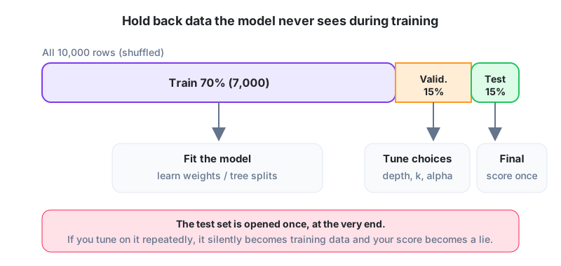
Measure a model on the rows it learned from and you're measuring memory, not skill. So you split your labelled data before training starts.

Set	Used for	How often you look at it
Training	fitting parameters (weights, splits)	every iteration
Validation	choosing between models and settings (depth, k, regularisation)	many times, during development
Test	the final, honest estimate of performance on new data	once, at the end

Two habits to build now. Shuffle before splitting, unless the data is a time series, where you split by date. And stratify classification splits so each set carries the same class balance.

The two failure modes

	Underfitting (high bias)	Overfitting (high variance)
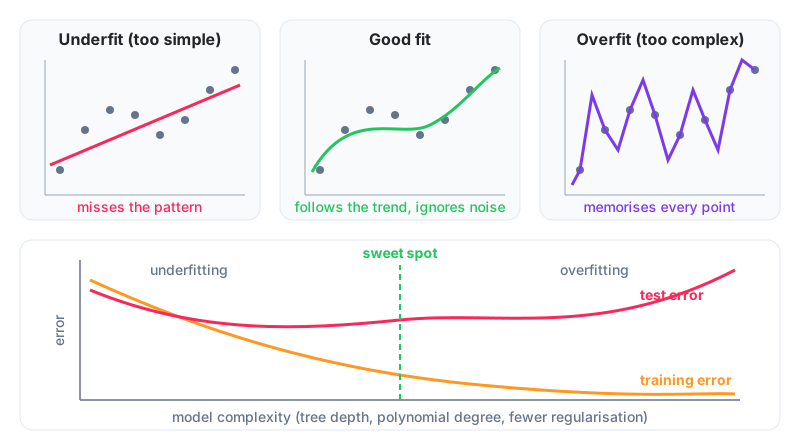
Symptom	training error high, test error high and similar	training error very low, test error much higher
Cause	model too simple, features missing	model too flexible, too few rows, noisy labels
Fix	add features, use a more flexible model, reduce regularisation	more data, simpler model, regularisation, early stopping, remove noisy features
Analogy	a student who only learned chapter 1	a student who memorised the answer key

The gap between training and test error is your overfitting gauge. Small gap with high error means underfitting. Large gap means overfitting. The bias-variance trade-off is just the observation that pushing complexity up lowers bias and raises variance, so the best model sits at the minimum of test error, never training error.

Reading the gap on a bakery model

A demand model for a Rawalpindi bakery was trained as a decision tree at several depths. RMSE is in loaves per day.

max_depth	Train RMSE	Validation RMSE	Gap	Verdict
1	42	44	2	underfit
3	28	31	3	better
5	19	24	5	best validation
8	9	29	20	overfitting begins
None (full)	0	38	38	memorised

Depth 5 wins, even though depth 8 and the unlimited tree look better on training data. Zero training error on the unlimited tree is the loudest warning sign there is. And notice the shape of the validation column. It falls, bottoms out, then rises, which is the curve in the diagram drawn with real numbers.

Regularisation: a penalty for complexity

Many models add a term to the loss that punishes large weights or deep trees. In linear models that's L2 (ridge) or L1 (lasso) with a strength alpha; in trees it's max_depth and min_samples_leaf; in boosting it's the learning rate and the number of trees. Tuning these on the validation set is how you walk to the sweet spot.

# run locally
from sklearn.model_selection import train_test_split
from sklearn.tree import DecisionTreeRegressor
from sklearn.metrics import mean_squared_error
import numpy as np

X_tr, X_te, y_tr, y_te = train_test_split(X, y, test_size=0.2, random_state=42)
for depth in [1, 3, 5, 8, None]:
    m = DecisionTreeRegressor(max_depth=depth, random_state=0).fit(X_tr, y_tr)
    tr = np.sqrt(mean_squared_error(y_tr, m.predict(X_tr)))
    te = np.sqrt(mean_squared_error(y_te, m.predict(X_te)))
    print(depth, round(tr, 1), round(te, 1), "gap", round(te - tr, 1))

Early stopping and ensembles

Iterative models (gradient boosting, neural networks) get more complex with every training round, so the number of rounds is itself a complexity knob. Early stopping watches validation error after each round and stops once it hasn't improved for, say, 50 rounds, then keeps the best round. It's the single most effective anti-overfitting tool for boosting, and the first thing we check when a student's boosted model has 2,000 trees and a suspicious training score. Averaging several models (an ensemble, such as a random forest) is the other big tool. Each model's random mistakes partly cancel, which lowers variance without raising bias. Both come back in lessons 9 and 11.

Is more data the answer? Plot a learning curve

Plot validation error against the number of training rows. Still falling? Collect more data. Flattened while training error stays low? More data won't close the gap, and you need a simpler model or better features. Both curves high and close together? You're underfitting, and data won't help either.

97% that turned into 71%: A Lahore e-commerce team built a return-prediction model with a deep random forest and reported 97% accuracy. Before launch the analyst split the data by month instead of randomly, and accuracy fell to 71%. The random split had put orders from the same customer on both sides, so the model was recognising customers, not learning behaviour. Splitting by customer, capping tree depth and adding min_samples_leaf brought training and test accuracy within three points of each other at 78%. Lower on paper, and real.

Before you move on

• Split before training. The test set is opened once, at the end.
• Underfitting means high error everywhere. Overfitting means low training error and much higher test error.
• The train-test gap is your gauge. Zero training error is a warning, not a win.
• Regularisation knobs (depth, alpha, leaf size, learning rate) move you along the complexity curve.
• Split by time or by entity whenever rows aren't independent.

Three things to try

1. A model shows training accuracy 99% and test accuracy 82%. Name the problem and three fixes.
2. A model shows training RMSE 500 and test RMSE 520 on a target whose typical value is 2,000. Name the problem and two fixes.
3. You have 3,000 loan applications from 2019 to 2024. Describe how you'd split them for a model that will be used in 2025, and why a random split is risky.