Time-Series Forecasting Basics

A distributor in Rawalpindi once showed us a demand forecast with a 4% error and asked why the trucks were still going out half empty. The forecast had been evaluated on shuffled data. Sales per day, electricity load per hour, cash withdrawals per week: much of business data is a sequence in time, and it breaks the usual ML assumption that rows are independent, because yesterday predicts today. This lesson shows you how to see the structure in a series, how to build honest baselines, and how to turn a series into a table so the algorithms you already know can forecast it.

See the structure first: decomposition

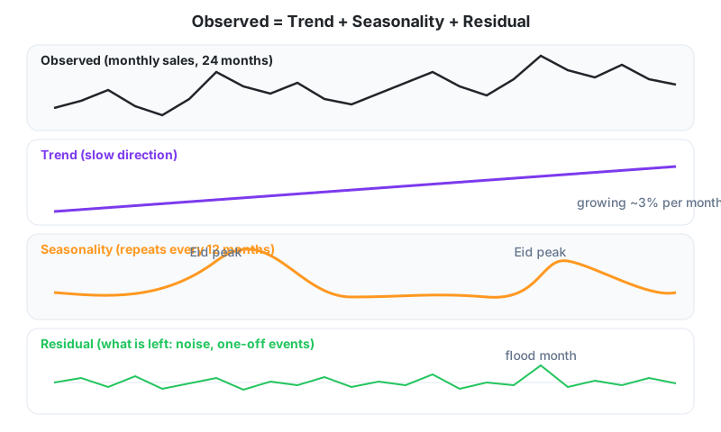
Component	What it is	Example
Trend	slow long-run direction	a Daraz seller growing 3% a month
Seasonality	a repeating pattern with a fixed period	Eid peaks, Friday dips, summer AC load
Cycle	slow waves without a fixed period	economic ups and downs
Residual	what is left after removing the above	a flood month, a viral post

Plot the series before you model anything. A quick decomposition (statsmodels.tsa.seasonal.seasonal_decompose) tells you whether seasonal features are needed and whether the pattern is additive or multiplicative (does the Eid bump grow as the level grows?).

Baselines you must beat

Three naive forecasts are surprisingly hard to beat, and a model that can't beat them has no business being deployed.

Baseline	Forecast for next period	When it is strong
Naive	last value	random-walk-like series (exchange rates)
Seasonal naive	value from one season ago (same month last year)	strongly seasonal series
Moving average	mean of the last n periods	noisy, slowly changing series

Three forecasts on one garment shop

Monthly sales (units) for a Lahore garment shop. We forecast months 7 to 9 using only earlier data, one step at a time.

Month	Actual	Naive (last)	MA-3 (mean of last 3)	Seasonal naive (12 months ago)
4	120
5	130
6	125
7	140	125	(120 + 130 + 125) / 3 = 125.0	128
8	160	140	(130 + 125 + 140) / 3 = 131.7	150
9	150	160	(125 + 140 + 160) / 3 = 141.7	145

Method	Absolute errors (m7, m8, m9)	MAE	MAPE
Naive	15, 20, 10	15.0	(10.7 + 12.5 + 6.7) / 3 = 10.0%
MA-3	15, 28.3, 8.3	17.2	(10.7 + 17.7 + 5.5) / 3 = 11.3%
Seasonal naive	12, 10, 5	9.0	(8.6 + 6.3 + 3.3) / 3 = 6.1%

Seasonal naive wins. That tells you the series is seasonal and that any decent model must carry last year's value as a feature. The moving average lags behind a rising trend, which is its classic weakness and the reason we rarely use it beyond a sanity check.

Turn the series into a supervised table

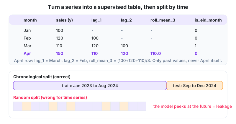
Build lag features (the value 1, 2, 7, 12 periods ago), rolling statistics (mean and std of the last 3, 7, 30 periods) and calendar features (month, weekday, is_eid_week, is_public_holiday), and every row becomes "features known before time t, target at time t". Gradient boosting, or even linear regression, can then forecast, and they often beat the classical models once you have extra drivers like price, promotions or weather.

Two rules that make or break this:

• No future in the features. A rolling mean for April must use only March and earlier.
• Split by time. Train on the past, validate on the following period, never shuffle. Use TimeSeriesSplit for CV.

Classical models in one table

Model	Idea	Use when
Exponential smoothing (Holt-Winters)	weighted average of the past with trend and seasonal terms	one clean series, few drivers, quick and stable
ARIMA / SARIMA	regression on past values and past errors, with differencing for trend	stationary-after-differencing series, statistical rigour needed
Prophet	trend + multiple seasonalities + holiday effects	daily business data with holidays, minimal tuning
Gradient boosting on lags	supervised learning on a lag table	many series, many external drivers (price, promo, weather)

# run locally
import pandas as pd
from sklearn.ensemble import GradientBoostingRegressor
from sklearn.metrics import mean_absolute_error

s = pd.read_csv("monthly_sales.csv", parse_dates=["month"]).set_index("month")["units"]
df = pd.DataFrame({"y": s})
for lag in [1, 2, 3, 12]:
    df[f"lag_{lag}"] = s.shift(lag)
df["roll_mean_3"] = s.shift(1).rolling(3).mean()     # shift(1): no future
df["month_num"] = df.index.month
df = df.dropna()

train, test = df[:-6], df[-6:]                      # last 6 months held out, in order
X_cols = [c for c in df.columns if c != "y"]
m = GradientBoostingRegressor(random_state=0).fit(train[X_cols], train["y"])
pred = m.predict(test[X_cols])
print("model MAE:", mean_absolute_error(test["y"], pred))
print("seasonal naive MAE:", mean_absolute_error(test["y"], test["lag_12"]))

Why the Eid flag beat every other feature: That Rawalpindi distributor supplies about 1,200 kiryana stores and forecasts weekly demand per product to plan truck loads. The first attempt used a random train/test split and reported MAPE 4%; a proper time-ordered split showed 19%. Rebuilt with lag features (1, 2, 4, 52 weeks), rolling means, an Eid-week flag from the Islamic calendar and the planned promotion list, a LightGBM model reached MAPE 11% against 16% for seasonal naive. That gain was worth roughly one fewer truck a day. The Eid flag explained more than any other feature, because both Eids shift 10 to 11 days earlier every year and the seasonal naive baseline kept missing them.

Quick recap

• Decompose first. Trend, seasonality and residual tell you which features you need.
• Seasonal naive and moving average are the baselines every forecast has to beat.
• Lag, rolling and calendar features turn forecasting into ordinary supervised learning.
• No future information in the features, and always split and cross-validate by time.
• Pakistani calendars matter. Eid, Muharram and budget season move every year and need explicit features.

Try this

1. Extend the worked example: month 10 actual is 170, and month 10 last year was 155. Compute the naive, MA-3 and seasonal naive forecasts for month 10 and their absolute errors.
2. List the features you'd build to forecast hourly electricity load for a Karachi feeder. Mark which are lags, which are calendar and which are external drivers.
3. Explain in two sentences why a random shuffle before splitting makes a time-series model look better than it is.