Introduction to pandas

What does a file of 2.3 million card transactions look like in Excel? A spinning cursor, then a crash. In pandas it's a variable. pandas is the library that made Python the default tool for data analysis, and it gives you the DataFrame, a table with named columns where one line does what took a loop and a dict in the previous lesson, on millions of rows. This lesson is a tour of the operations you'll use daily. pandas isn't in the standard library, so run these examples locally after pip install pandas (Lesson 25 covers virtual environments).

Series and DataFrame

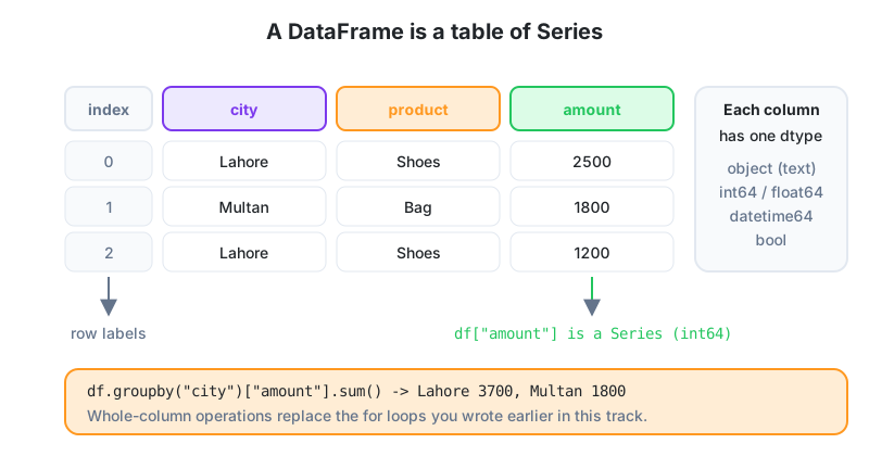
A Series is one column, values plus an index. A DataFrame is a dict of Series sharing the same index. Most of the time you'll build one from a file.

import pandas as pd

df = pd.DataFrame({
    "city":    ["Lahore", "Multan", "Lahore", "Karachi", "Lahore"],
    "product": ["Shoes", "Bag", "Shoes", "Watch", "Bag"],
    "amount":  [2500, 1800, 3200, 9100, 1500],
    "sold_on": ["2026-09-01", "2026-09-01", "2026-09-02", "2026-09-02", "2026-09-03"],
})
print(df)
print(df.shape)          # (5, 4)  rows, columns
print(df.dtypes)         # object, object, int64, object

For a real file, df = pd.read_csv("sales.csv"). pandas reads the header, guesses column types and handles quoting. pd.read_excel("file.xlsx") works once openpyxl is installed.

Looking at data

print(df.head(3))              # first rows
print(df.info())               # columns, non-null counts, dtypes, memory
print(df.describe())           # count, mean, std, min, quartiles, max for numeric columns
print(df["city"].value_counts())
print(df["amount"].sum(), df["amount"].mean(), df["amount"].median())

Compare this with Lesson 21. value_counts() is Counter, and describe() is the whole statistics module, one call each. We insist that every new file gets info() and describe() before any analysis, because that's where you discover the amount column loaded as text.

Selecting rows and columns

print(df["amount"])                        # one column, a Series
print(df[["city", "amount"]])              # several columns, a DataFrame
print(df[df["amount"] > 2000])             # filter rows with a boolean mask
print(df[(df["city"] == "Lahore") & (df["amount"] > 2000)])   # & not 'and', brackets required
print(df.loc[0, "city"])                   # by label: row 0, column city
print(df.iloc[-1])                         # by position: last row

The filter df[df["amount"] > 2000] is the pandas version of a list comprehension with an if. Inside a mask, combine conditions with &, | and ~, and put each part in parentheses. Leaving out the parentheses gives an error message that has confused every student we've taught.

Adding and transforming columns

df["with_gst"] = df["amount"] * 1.17                       # whole column at once
df["sold_on"] = pd.to_datetime(df["sold_on"])              # text to real dates
df["weekday"] = df["sold_on"].dt.day_name()
df["size"] = df["amount"].apply(lambda a: "big" if a > 2500 else "small")
df["city"] = df["city"].str.upper()                        # string methods via .str
print(df)

No loops. Arithmetic on a column applies to every row (this is vectorisation, and Lesson 23 explains why it's fast). The .dt and .str accessors expose the datetime and string methods you already know.

Group-by and aggregation

print(df.groupby("city")["amount"].sum())
print(df.groupby("city")["amount"].agg(["count", "sum", "mean"]))
print(df.groupby(["city", "product"])["amount"].sum().reset_index())
print(df.pivot_table(index="city", columns="product", values="amount", aggfunc="sum", fill_value=0))

groupby is the Lesson 21 defaultdict loop. pivot_table is the Excel pivot you already know, with rows, columns and an aggregation.

Sorting, missing values and joins

print(df.sort_values("amount", ascending=False).head(3))

print(df.isna().sum())                     # missing values per column
df["amount"] = df["amount"].fillna(0)      # or df.dropna(subset=["amount"])

cities = pd.DataFrame({"city": ["LAHORE", "MULTAN", "KARACHI"], "province": ["Punjab", "Punjab", "Sindh"]})
merged = df.merge(cities, on="city", how="left")     # SQL-style join
print(merged.groupby("province")["amount"].sum())

Saving results

merged.to_csv("sales_enriched.csv", index=False)
merged.to_excel("sales_enriched.xlsx", index=False)      # needs openpyxl

How pandas maps to what you know

Task	Pure Python (Lessons 8-21)	pandas
Read CSV	csv.DictReader loop	pd.read_csv()
Filter rows	list comprehension with if	df[mask]
New column	loop and assign	df["x"] = ...
Count values	Counter	value_counts()
Group and sum	defaultdict loop	groupby().sum()
Join two tables	dict lookup in a loop	merge()
Summary stats	statistics	describe()

Back to those 2.3 million transactions: A fraud analyst at a Karachi bank gets that file every month. With pandas she loads it in about twenty seconds, filters to night-time foreign transactions above Rs 50,000, groups by card to find cards with more than five such transactions, and merges with the customer table to attach branch and phone. The whole notebook is around 25 lines and reruns every morning on the new file.

Your first five commands

On any new file, run read_csv, head, info, describe and value_counts, in that order. After that, remember that a DataFrame is a table whose columns are Series with one dtype each, that you filter with boolean masks joined by & and | in parentheses, that you operate on whole columns rather than looping, and that groupby, pivot_table and merge replace the dict patterns from Lesson 21. pandas isn't in the playground, so install it locally in a virtual environment.

Run these locally

1. Build the DataFrame above, add a discounted column at 10% off, and print total revenue per city sorted descending.
2. Create a second DataFrame of product costs, merge it in, compute margin per row and the average margin per product.
3. Read any CSV you have (or export one from Excel), run info() and describe(), and write down two data-quality problems you notice.

print("Hello from CSA!")

for i in range(5):
    print(i * i)